The other evening I was deep down a rabbit hole. It started with a simple question for ChatGPT:

“Please explain to me and educate me on how ZML works. What are its benefits and drawbacks? I really want to understand here”

After some back and forth I quickly realized I’d only understand this by building it. So I built a minimal (but working) version of ZML in Rust. The best way I know to understand something is to build it, and I wanted to distill what I learned into this blog so you could learn it too.

I’ll start this blog by going through how ZML works under the hood. Explain the end-to-end pipeline from model definition to StableHLO to PJRT. Once we have a solid understanding of what it should look like, we’ll build a toy/educational ML framework. The first version will be ugly, and the last part of this blog is devoted to cleaning it up.

What we’ll cover:

Part 1: Reading — how ZML works under the hood
Part 2: Building — building a toy framework that emits StableHLO
Part 3: Running — compiling and executing via PJRT
Part 4: Cleaning — making the API feel like a real framework
Demo — running SmolLM2-135M end to end

The outcome of this blog is that we’ll build a toy/educational ML framework, that will run the SmolLM2-135M model, something like this:

❯ ./target/release/examples/smollm2 chat                                                       
No compiled artifact given, compiling from scratch (seq=256)...
Compiled in 728.99ms
Loaded weights in 91.99ms

SmolLM2-135M-Instruct ready. Type a message and press Enter. Type "exit" to quit.

You> Hi 👋
Assistant> Hello! I'm here to help with any creative writing needs. What's on your mind?
[24 prompt tokens, 19 generated | TTFT 306ms | 4.5 tok/s]

I assume you’re comfortable with programming and have a basic understanding of neural networks: you know what a forward pass, a matmul, and a weight tensor are. You don’t need to be an expert, but I’ll cut to the chase pretty quickly.

What’s ZML?

ZML is an ML framework focused on inference, written in Zig. It lives at roughly the same level as PyTorch, but its design is fundamentally different: it’s based on a graph-compile-run pipeline. You stage a computation into a graph, compile it, and run the compiled artifact. There is no eager mode.

In PyTorch, the default is eager execution: ops run as you call them. It’s more like traditional Python code where things execute how they were written in the code. This is nice for model development, which is more like research. But when you want to turn it into a stable production artifact, you typically have to introduce a second stage (export, trace, compile), and that step is where weird edge cases show up. JAX is closer to ZML in spirit, you write code meant to be traced and compiled via XLA.

If you’re coming from a PyTorch world, three things stand out:

Graph-first: ZML builds a model as a staged computation graph. No hidden control flow, no dynamic dispatch at inference time.
Model and weights are separate: you can trace, validate, and compile the model structure without loading weights. When weights are tens of gigabytes, this separation gives you fast compile/test loops.
Cross-compilation: because the output is a compiled artifact targeting a backend, you can build once and run on CPU, GPU, or TPU without rewriting your serving stack.

As someone who has worked with inference for a long time, this really hits home. And I really wanted to understand how it works. Let’s get a high-level overview of how ZML works, and then we’ll dive into building out each part ourselves.

Part 1: Reading

The stack

There’s a big stack involved here and it’s not immediately obvious what does what. But nothing here is difficult per se, there’s just a lot of it.

The short version is:

Write the model in Zig, lower it to StableHLO (an MLIR dialect), then let OpenXLA compile/run it through PJRT

Before we unpack each layer, here’s the short explanation of each piece:

StableHLO is an IR (intermediate representation) that describes ML computations. It’s a dialect of MLIR, so in many places, including this blog, they’re used interchangeably.
PJRT is the runtime API that compiles and executes those computations on actual hardware.
OpenXLA is the umbrella project that ties them together.

The top of the stack is the easiest to understand, since it feels very similar to PyTorch. You write your model in Zig as a struct:

const Scale = struct {
    weight: zml.Tensor,

    pub fn forward(self: Scale, x: zml.Tensor) zml.Tensor {
        return self.weight.mul(x);
    }
};

The struct has a weight tensor and a forward method that does an elementwise multiply. You’d use it like:

const x = zml.Tensor.init(.{1, 4}, .f32);
const y = scale.forward(x);

This is somewhat pseudo-code, but you get the idea.

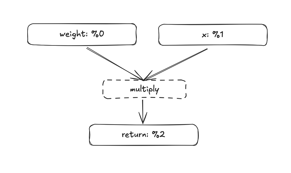
The core part to understand here is that there’s no data attached to this yet. The data in the weight tensor isn’t here, and it doesn’t need to be. In ZML a tensor is just some shape metadata plus an MLIR value that identifies the operation that produced it.

“What the hell is an MLIR value?”, fair question. It’s tempting to first think of it as a pointer to data in memory. But it’s not that since there’s no data to point to. Think of it as a name for a result. It’s what’s called a single static assignment (SSA) value: each operation in the computation graph produces one or more results, and each result gets a unique SSA name (like %0, %4). The operation itself is the node in the graph; the SSA value is the handle you use to refer to its output. In essence, it tells you where a tensor came from and how it flows through the computation, but it doesn’t hold actual numeric data.

Let’s visualize our multiplication. Both the weight and the input tensor x are tensors, so they get assigned an SSA value. Simply %0 and %1. In the forward pass the two values are multiplied, producing a new tensor with the id %2. So the new tensor with the id %2 is just the result of whatever came from multiplying %0 and %1.

If the MLIR value doesn’t fully click yet, don’t worry, it will become clearer as we go deeper and start building things ourselves.

What’s MLIR really?

MLIR (Multi-Level Intermediate Representation) is a compiler infrastructure for building IRs. It provides the core machinery like types, operations, optimization passes, and lets you define “dialects” on top of it. StableHLO is one such dialect. When you see “MLIR” in the ZML context, it usually means “the framework that StableHLO is built on,” not a separate layer.

StableHLO

One layer under the ZML graph we have StableHLO (HLO standing for High Level Operations). StableHLO is an intermediate representation for ML computations. It’s an MLIR dialect, which is why “StableHLO” and “MLIR” are sometimes used interchangeably. The common confusion is to think StableHLO is MLIR, when really StableHLO is a vocabulary of operations defined within the MLIR framework.

The core value proposition is that StableHLO defines a standard, portable set of operations, like stablehlo.add, stablehlo.dot_general, stablehlo.broadcast_in_dim, etc. Plenty of frameworks already use StableHLO, like JAX. There’s even a PyTorch XLA backend that works similarly. So what ZML is doing isn’t entirely new, the difference is that ZML makes this the default and only path.

The StableHLO of our elementwise multiplication would look something like this:

module {
  func.func @main(%0: tensor<1x4xf32>, %1: tensor<1x4xf32>) -> tensor<1x4xf32> {
    %2 = stablehlo.multiply %0, %1 : tensor<1x4xf32>
    return %2 : tensor<1x4xf32>
  }
}

Not the nicest thing to read, but still pretty understandable. tensor<1x4xf32> is a 1x4 tensor of 32-bit floats, assigned to SSA value %0. This would be our weights. And the other 1x4 tensor with id %1 is x. The tensor with the id %2 is whatever that comes out of the instruction stablehlo.multiply, where %0 and %1 are arguments to that function. And we can infer that %2 has the shape 1x4 as well.

We’re building up a compute graph of the entire thing, all without actual data. As long as we know the shapes, this works.

Caveat

StableHLO does actually support dynamic shapes. E.g. unknown batch size tensor<?x4xf32> but this is exactly something we’d like to avoid to be able to compile ahead of time. ZML doesn’t support it either and we’ll skip it for our educational ML framework as well.

You might have noticed that our ZML code didn’t specify any shapes for the weight tensor. Only x was defined as zml.Tensor.init(.{1, 4}, .f32);. So how did it become 1x4 in this case? We’ll address this later when we build our own framework, but to peek into the future a bit: ZML (and our future framework) actually looks at the header of a .safetensor file to determine the final shapes of the weight tensor. All .safetensor files have a JSON part at the start of the file containing each tensor’s name, dtype, shape, and byte offsets, all before the actual data blob. Our struct tells us what tensors our model consists of, and we map this to a .safetensor file which then tells us the final exact shape of everything.

This means that our modelling code is more flexible, the same model definition works for a 7B and 13B model. But we can still trace and compile the entire graph by just reading a few kilobytes of data, without loading the model weights.

PJRT

The last missing piece is how this actually gets executed on a machine. StableHLO is just an IR, it can’t run by itself. The missing piece is PJRT. PJRT is honestly a big beast to tackle and I’ve just scratched the surface, but the key part to understand is that PJRT defines a compilation entrypoint and different plugins (for GPU, CPU, TPU, etc.) do the heavy lifting.

In simple terms: we hand the StableHLO text to PJRT, and if we target CPU, the plugin goes through LLVM and produces native machine code. This is how our ZML defined multiply becomes something that actually runs on a computer.

Part 2: Building

In this part we’ll build a small ML framework that lets us:

Build a high-level graph describing some computation
Turn that graph into valid StableHLO
Hand that StableHLO to PJRT and execute the graph on CPU

To keep the scope small, we’ll focus only on a simple y = x·w + b layer. First we’ll build the graph and emit StableHLO. The API will be ugly and nothing like PyTorch or ZML. Then we’ll wire up PJRT to actually execute it. In part 4 of the blog, we’ll clean up the API to something that feels more like a real framework.

If we jumped straight to the nice API, we’d miss the learning. There’s a fair amount of quality-of-life work that frameworks like PyTorch and ZML do that, while satisfying to build, can obscure the underlying concepts.

All the code is available at github.com/ErikKaum/fusebox.

Building tensors

I’m calling this library fusebox: box since it’s small, fuse since there’s still some fire in this.

We’ll start with four small modules. These are simple, but having good intuition around them matters:

src/dtype.rs: just F32 for now, with a method to print the MLIR string ("f32")
src/shape.rs: Shape { dims: Vec<i64>, dtype: DType } dimensions plus dtype, with a method to produce the MLIR tensor type string (e.g. tensor<2x4xf32>)
src/value.rs: ValueId(u32) the SSA id in the graph. Instead of storing it as a string, like "%5", everywhere, we store the integer and only render it when printing
src/tensor.rs: Tensor { shape: Shape, value: ValueId } the core building block that combines all of the above

The tensor is essentially a symbolic handle. When you’ll do something like matmul(x, w), the builder (which we’ll build next) will:

allocate a fresh ValueId
append an instruction saying “this new value id is the result of DotGeneral(lhs=x.value, rhs=w.value, …)”
and return a new Tensor pointing at that id

Which is exactly the same process that we had previously, in the elementwise multiplication example. No data, just a reference to a result in the computation graph.

I won’t go through exactly all of the code since it would be way too verbose, but I’ll show code examples with the aim that it’ll improve your intuition around this.

To reiterate: a tensor has a shape, in this case 1x4, a datatype, and the SSA Value attached to it. This is how our high level Rust struct maps very directly to StableHLO.

A tensor t like this:

let t = Tensor {
    shape: Shape {
        dims: vec![1, 4],
        dtype: DType::F32,   // → "f32"
    },
    value: ValueId(3),       // → "%3" in the StableHLO output
};

Would be represented like this in StableHLO:

%3 : tensor<1x4xf32>
 ^         ^  ^ ^
 |         |  | └── DType::F32
 |         dims: [1, 4]
 ValueId(3)

Building graphs

Now we’re ready to start connecting tensors together into a graph.

First, we’ll make our own intermediate representation (IR) in Rust, which then gets converted into StableHLO. “Another IR?!”, I hear you say. Bear with me. ZML for example doesn’t have its own IR, its tensors get directly converted into StableHLO, and that’s probably what you’d do for a real framework. But for learning purposes, having a thin Rust representation of the graph before converting it to StableHLO lets us separate the logic of building the graph from the concerns of StableHLO syntax. And I really don’t want to write a blog about StableHLO syntax.

So we’ll have three new modules:

src/ir.rs: defines functions, parameters, and instructions
src/print_mlir.rs: takes our internal IR and prints it as StableHLO
src/builder.rs: defines a FuncBuilder that ties tensors together into a graph

Let’s walk through this carefully, since there’s a handful of moving parts here.

At the top level we have a module, which contains a list of functions. Think of a module as the entrypoint, in our case, the top-level forward of a neural network.

A function has three parts:

Parameters — the inputs to the function, each with an SSA value
Instructions — the operations inside the function, each producing an SSA value
A return value — an SSA value that becomes the output

To give an overview, these are the main structs & enums we’re working with:

pub struct Module {
    pub functions: Vec<Function>,
}

pub struct Function {
    pub name: String,
    pub params: Vec<Param>,
    pub insts: Vec<Stmt>,
    pub ret: Option<ValueId>,
}

pub struct Param {
    pub name: String,
    pub shape: Shape,
    pub value: ValueId,
}

pub struct Stmt {
    pub result: ValueId,
    pub inst: Inst,
}

pub enum Inst {
    DotGeneral(DotGeneral),
    BroadcastInDim(BroadcastInDim),
    Add(Add),
}

So each Inst variant (like DotGeneral, Add and BroadcastInDim) carries the ValueIds of its inputs plus the output shape. If we look closer at the Add instruction:

#[derive(Debug, Clone)]
pub struct Add {
    pub lhs: ValueId,
    pub rhs: ValueId,
    pub out: Shape,
}

And let’s say our left hand side has the value id 0 and the rhs has id 1. Then we could look at the shape and dtype of tensors 0 and 1 respectively, and produce the following StableHLO:

"stablehlo.add"(%0, %1) : (tensor<1x4xf32>, tensor<1x4xf32>) -> tensor<1x4xf32>

This is how we essentially keep a mapping of each StableHLO instruction, and have a corresponding Rust struct for each one of them. Later we’ll also see how we explicitly set the output shape and dtype.

If this doesn’t fully make sense yet, I’d encourage reading it once more. Having a solid understanding of the IR made everything else click for me.

The full IR definitions are in the repo, they’re straightforward once you see the pattern.

Building builders

Now the builder. We’ll create a struct called the FuncBuilder. Each instruction we defined in the IR gets a corresponding method on the FuncBuilder: builder.add(...), builder.dot_general(...), builder.broadcast_in_dim(...), and so on.

But before those, let’s look at the fresh() method. This will be the function that gives fresh ValueIds, and essentially the way we do bookkeeping of the ids. It’s pretty simple, just incrementing a counter. But note that this also makes the FuncBuilder stateful. If we change the order from add(x, y) to add(y, x), the result is the same since addition is commutative, and the result tensor gets the same ValueId either way. But x and y themselves will get swapped ValueIds, whichever is added to the graph first gets the lower id. That means ValueIds aren’t a stable way to reference a tensor: the same logical tensor can end up with different ids depending on construction order. It’s fine for now, but this will come up later as a real issue when we want to produce a stable ABI on top of ValueIds.

pub struct FuncBuilder {
    func: Function,
    next_id: u32,
}

impl FuncBuilder {
    
    fn fresh(&mut self) -> ValueId {
        let id = self.next_id;
        self.next_id += 1;
        ValueId(id)
    } 
    
    pub fn matmul_2d(&mut self, x: &Tensor, w: &Tensor) -> Result<Tensor, Error> {
        ...
    }

    pub fn broadcast_bias_1d(&mut self, b: &Tensor, batch: i64) -> Result<Tensor, Error> {
        ...
    }

If we dive deeper in how the add() is actually implemented, we’ll find that most of the ceremony is validating shapes and dtypes. Which I’ve omitted in this blog. But the core pattern is always the same:

pub fn add(&mut self, a: &Tensor, b: &Tensor) -> Result<Tensor, Error> {
    // ... shape/dtype validation ...

    let out_shape = a.shape.clone(); // how we manually determine output shapes
    let result = self.fresh();  // allocate a new ValueId (just a counter)

    self.func.insts.push(Stmt {
        result,
        inst: Inst::Add(Add {
            lhs: a.value,
            rhs: b.value,
            out: out_shape.clone(),
        }),
    });

    Ok(Tensor::new(out_shape, result))
}

We call self.fresh() which gives us a new id. Then we create a new statement: this value id is the result of the add instruction on the two inputs. We append it to the function’s instruction list and return a new Tensor pointing at the result.

The matmul_2d and broadcast_bias_1d methods follow the exact same pattern: validate shapes, allocate a fresh ValueId, push a statement, return a new Tensor. To keep things simple I’ve kept the methods specific to a certain dimension, so matmul_2d instead of just matmul, we’ll relax this later. Here you’ll find the full builder code.

If this doesn’t 100% click yet, this example should help. Here’s the full y = x·w + b layer built with the current API of our framework:

let mut f = FuncBuilder::new("main");

let x = f.param("x", Shape::new(vec![2, 4], DType::F32));   // -> %0
let w = f.param("w", Shape::new(vec![4, 3], DType::F32));   // -> %1
let b = f.param("b", Shape::new(vec![3], DType::F32));      // -> %2

let y = f.matmul_2d(&x, &w)?;                               // -> %3
let bb = f.broadcast_bias_1d(&b, 2)?;                       // -> %4
let out = f.add(&y, &bb)?;                                  // -> %5

f.ret(&out);

let func = f.finish();
let module = Module { functions: vec![func] };
println!("{}", print_module(&module));

We instantiate the FuncBuilder, add three parameters (x, w, b), chain a matmul, a broadcast, and an add, set the return, and finish. Essentially the same thing as in this graph:

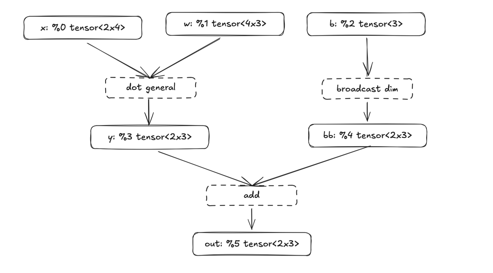
Each f.param() call does two things:

it allocates the next ValueId to each tensor, this is how x becomes %0 and
and registers the tensor as a function input

So our three params become the function signature @main(%0: …, %1: …, %2: …), while the intermediate tensors (%3, %4) are produced by operations in the function body. The final result %5 is what gets returned. Once we print it, we get StableHLO (truncated for readability):

module { 
    func.func @main(%0: tensor<2x4xf32>, %1: tensor<4x3xf32>, %2: tensor<3xf32>) -> tensor<2x3xf32> {
        %3 = stablehlo.dot_general ...
        %4 = stablehlo.broadcast_in_dim ...
        %5 = stablehlo.add %3, %4 : tensor<2x3xf32>
        return %5 : tensor<2x3xf32> 
    } 
}

We can save this text as a .mlir file and use a tool from the StableHLO repo to verify that the output is valid. Running stablehlo-opt forward.mlir, will catch any syntax or type errors.

So far we’ve:

Created a high-level way of representing tensors with shapes and dtypes
Built a small IR that can represent basic StableHLO operations
Tied them together with a function builder that creates a computation graph
Printed the graph as StableHLO

If you think the API feels weird compared to PyTorch or ZML, you’re not alone. We’re calling methods on a builder rather than doing tensor.add(). In part 4 we’ll clean this up and start building layers on top of the FuncBuilder, which will make the API feel more like a modern ML framework.

But this actually works! It produces real StableHLO, which means that we can move to the next part of the pipeline: compile it with PJRT and actually run it.

Part 3: Running

We’re finally getting close to producing something. After all this plumbing, we’ve reached the step of actually executing a computation graph. If you’ve so far felt that we’re not doing much: “it’s just a StableHLO wrapper, right?”, you’ll start to feel it now.

In plain terms, we now have a program that produces StableHLO (basically a text file). We’ll hand this text file to another program, wire up the correct inputs, compile it, and run it. To really drive home the “two programs” point, I first wrote this runner in Go. There’s no need for the graph-builder and the runner to be in the same language, and using a different one makes the separation palpable.

Quick and dirty in Go

We’ll use a Go package called go-xla. The painful part of working with PJRT directly is keeping track of plugin versions (which you don’t have to do in ZML), go-xla handles this with an installer.AutoInstall() function that auto-downloads the correct precompiled PJRT plugin for your platform.

The flow has essentially these three steps: 1) read the MLIR file 2) compile it and 3) execute it with input buffers.

func main() {
    // 1. Auto-download PJRT plugin
    installer.AutoInstall("", true, installer.Normal)

    // 2. Read StableHLO and compile it
    mlirBytes, _ := os.ReadFile("forward.mlir")
    plugin, _ := pjrt.GetPlugin("cpu")
    client, _ := plugin.NewClient(nil)
    exec, _ := client.Compile().WithStableHLO(mlirBytes).Done()

    // 3. Create input buffers with REAL DATA and execute
    x := []float32{1, 2, 3, 4, 5, 6, 7, 8}
    w := []float32{1, 0, 0, 0, 1, 0, 0, 0, 1, 1, 1, 1}
    b := []float32{10, 20, 30}

    bx, _ := pjrt.ArrayToBuffer(client, x, 2, 4)
    bw, _ := pjrt.ArrayToBuffer(client, w, 4, 3)
    bb, _ := pjrt.ArrayToBuffer(client, b, 3)

    outs, _ := exec.Execute(bx, bw, bb).Done()
    outFlat, outDims, _ := pjrt.BufferToArray[float32](outs[0])

    fmt.Printf("output dims=%v\n", outDims)
    fmt.Printf("output flat=%v\n", outFlat)
}

Note the key moment: only now, at ArrayToBuffer, do we pass real data. Everything before this was purely symbolic. The full Go code with proper error handling is in the fusebox repo.

And once you run this with go run main.go you’ll get:

output dims=[2 3]
output flat=[15 26 37 23 34 45]

If you’ve come this far, you should congratulate yourself. You’ve understood the entire pipeline from start to finish. Everything from here onwards enhances and polishes this pipeline, but conceptually we won’t change anything fundamental. This is it. But don’t be fooled, there’s still tons of work to do before we can call this a toy ML framework.

Moving the runner to Rust

The obvious shortcoming is that we can’t handwrite input arrays in Go for every StableHLO program. As a silly solution, we could create a json file that would describe the inputs with shapes and dtypes. We’d have to generate this in the Rust code, and hand it over to the Go runner. Something like this:

{
  "entry": "main",
  "inputs": [
    {"name": "x", "dtype": "f32", "shape": [2,4]},
    {"name": "w", "dtype": "f32", "shape": [4,3]},
    {"name": "b", "dtype": "f32", "shape": [3]}
  ],
  "outputs": [
    {"dtype": "f32", "shape": [2,3]}
  ]
}

But wouldn’t it be nice if the runner could infer the shapes and dtypes from the builder’s params. Rather than having to type out things twice: once for building the graph and a second time for passing real data to the graph.

We’ll do this but not quite yet. First we need to have a runner in Rust. We’ll use the pjrt crate which doesn’t have an autoinstaller like go-xla. Fortunately, ZML maintains a pre-compiled repo, of the pjrt plugins. It took some trial and error to find which plugin version corresponds to the rust bindings. Version 0.2.2 at least seems to match. Again, you don’t have to think about this with ZML.

When moving the runner to Rust we have an API that looks like this. We still set up host buffers manually:

fn main() -> Result<(), String> {
    let mlir = build_your_stablehlo_mlir_string();

    let runner = PjrtCpuRunner::from_mlir_text(&mlir, default_cpu_plugin_path())?;

    let x = HostTensorF32::new(vec![2, 4], vec![1.,2.,3.,4.,  5.,6.,7.,8.])?;
    let w = HostTensorF32::new(vec![4, 3], vec![1.,2.,3., 4.,5.,6., 7.,8.,9., 10.,11.,12.])?;
    let b = HostTensorF32::new(vec![3], vec![1., 2., 3.])?;

    let y = runner.run_f32(vec![x, w, b])?;
    println!("output dims={:?}", y.dims);
    println!("output flat={:?}", y.data);

    Ok(())
}

Link to the full code.

At this point we have a complete pipeline entirely in Rust: define the graph, emit StableHLO, compile via PJRT, execute, and get results back. The API is rough, but it works.

The next part is about making it feel like a real framework.

Part 4: Cleaning

So far we’ve built a framework that takes high level tensors, builds a computation graph in StableHLO, compiles it via PJRT, and executes it on CPU. It works, but the API leaves a lot to be desired. We’ve been optimizing for learning instead of ergonomics, and now it’s time to make this feel like a real framework.

If you’ve made it this far, you already have a solid understanding of the stack that ZML builds upon: which is the main goal of this blog. Feel free to call it a day. But if you’re curious about the long tail of details that make a framework usable rather than just correct, read on. Nothing here changes the fundamentals, but these are the edges that separate a StableHLO wrapper from something you’d actually want to use.

From graph plumbing to model code

The FuncBuilder approach felt like building “from the outside.” We pushed parameters into a builder, called graph-building helpers, and printed a StableHLO function. This was great for learning, but the code that describes a model doesn’t look like a model: it looks like graph plumbing.

The shift we want to do is to go from manually constructing a graph, to automatically tracing a forward pass. Enter the TraceCx (tracing context). You write a forward pass once, and it runs in a mode where tensor operations don’t compute, instead they’re recorded. Similarly to what’s done in ZML or JAX.

pub struct TraceCx {
    builder: Rc<RefCell<FuncBuilder>>,
    prefix: String,
}

The TraceCx wraps our FuncBuilder and adds two key things:

hierarchical name scoping (the prefix)
and a distinction between input parameters and weight parameters

We’ll see why both of these matter shortly.

With TraceCx, a linear layer becomes a struct with a forward method. This looks a lot more like the modelling code we’re familiar with from PyTorch. The big difference is that we’re still manually writing the trace_init() method.

pub struct Linear {
    pub w: Tensor,
    pub b: Option<Tensor>,
}

impl Linear {
    pub fn trace_init(cx: &mut TraceCx, name: &str, in_dim: i64, out_dim: i64, bias: bool) -> Self {
        let _s = cx.push_scope(name);
        let w = cx.weight("w", Shape::new(vec![in_dim, out_dim], DType::F32));
        let b = if bias {
            Some(cx.weight("b", Shape::new(vec![out_dim], DType::F32)))
        } else {
            None
        };
        cx.pop_scope(_s);
        Self { w, b }
    }

    pub fn forward(&self, cx: &mut TraceCx, x: &Tensor) -> Result<Tensor, Error> {
        let y = cx.matmul_2d(x, &self.w)?;
        if let Some(b) = &self.b {
            let batch = x.shape.dim(0);
            let bb = cx.broadcast_bias_1d(b, batch)?;
            cx.add(&y, &bb)
        } else {
            Ok(y)
        }
    }
}

You’d use it like this:

let mut cx = TraceCx::new("main");

let x = cx.input("x", Shape::new(vec![2, 4], DType::F32));
let proj = Linear::trace_init(&mut cx, "proj", 4, 3, true);
let y = proj.forward(&mut cx, &x)?;

cx.set_ret(&y);
let func = cx.finish();

In practice, TraceCx is a nicer façade over the same essentials the builder had: it owns the function-under-construction, hands out ValueIds, provides ops, and produces StableHLO. The important shift is where the model logic lives. A module is a struct with weight fields; forward is a method that composes ops; tracing works by calling forward once with symbolic tensors.

That might just look like semantic changes, but it’s the first step from “graph construction code” into “model code.” And later, we can extract this pattern into a proc-macro, which is really when it starts to feel like magic.

Signatures: the bridge to PJRT

Now that we’ve cleaned up how the graph gets constructed by having a TraceCx, let’s look at the next step.

Remember, the last line from the previous example:

let func = cx.finish();

func holds the StableHLO text that we want to pass to the PJRT runtime.

But we’re still manually creating HostTensorF32 values that match the graph. Let’s fix that. Instead, we want the TraceCx to produce a structured signature that the runtime can use directly.

pub struct ParamSpec {
    pub name: String,
    pub shape: Shape,
    pub value: ValueId,
    pub kind: ParamKind,
}

pub struct Signature {
    params: Vec<ParamSpec>,
    by_name: HashMap<String, usize>,
}

The Signature is extracted from the traced parameters: name, shape, dtype, and whether it’s an input or a weight. It becomes the single source of truth for runtime binding. The runner can validate inputs, pack them in the correct argument order, and later separate which parameters are the model weights (which need to be bound once) from which parameters are the inputs (bound per request).

let runner = PjrtCpuRunner::from_function(&func, default_cpu_plugin_path())?;

let mut ins = runner.inputs();
ins.set("x", vec![1., 2., 3., 4., 5., 6., 7., 8.])?;
ins.set("proj/w", vec![1., 0., 0., 0., 1., 0., 0., 0., 1., 1., 1., 1.])?;
ins.set("proj/b", vec![10., 20., 30.])?;

let y = runner.run(ins)?;

Concretely what happens, is that we pass the &func into the PjrtCpuRunner::from_function(...) and then we can set the vectors as the runner inputs. Through ins = runner.inputs() and ins.set(). This is an improvement, but we’re still not reading proj/w and proj/b from a safetensor file. And the inputs x are still bound to the runner the same way as the weights. But we’re getting there.

Notice the scoped names: "proj/w" and "proj/b" came from the cx.push_scope("proj") call in trace_init(). We’re starting to see the real difference between the TraceCx and the old FuncBuilder: the tracer produces an ABI, not just a graph.

Stable names and param kinds

Now that the tracer produces an ABI, we need to be more careful about naming. Remember the ValueId instability we discussed in Part 2? The SSA value id is not a stable identifier: add a new layer and all the indices shift. For an ABI, we need names that come from the model structure and match the checkpoint.

What we already saw earlier with the proj suffix, is the result of the push_scope/pop_scope mechanism, which gives us hierarchical names: a Linear inside an MLP named "proj" gets weights named "proj/w" and "proj/b". These names are stable. They don’t change when you reorder operations, and they naturally match the naming conventions in safetensors weight files.

The practical approach is to align the naming of the struct fields (tensors) with the weight file. Meaning that the ultimate goal is that we can directly align the weights in a safetensor file to the tensors in our model. In a later section I’ll add a rename macro #[module(name = "new_name")], for inevitable mismatches. Which is another one of these quality-of-life things you’d want in a real ML framework. But for now, we assume that the names are the same in the safetensor files as in the struct fields.

The other important distinction is ParamKind:

pub enum ParamKind {
    Input,
    Weight,
}

From the graph’s point of view, all parameters are the same, just nodes. But from a model’s point of view, there’s a clear difference. Inputs are a runtime contract, they change per request. Weights are a checkpoint contract, loaded once. This separation matters because in a real serving system, the hot path is request execution. You bind weights once at startup and rebind inputs per request.

With this change we can avoid doing everything through the ins.set() which we did above.

Where do weight shapes come from?

Tracing requires knowing exact tensor shapes. And so far we’ve supplied those shapes manually like:

let proj = Linear::trace_init(&mut cx, "proj", 4, 3, true);

where 4 and 3 become the in and out dimensions.

let w = cx.weight("w", Shape::new(vec![in_dim, out_dim], DType::F32));

Obviously, this is not the way.

ZML’s answer: read the shapes from the checkpoint file’s metadata, compile the graph from shapes alone, and load the actual weight data separately (or in parallel). Importantly, we can compile the graph from just the shapes and dtypes, we don’t need to load the entire safetensor file into memory for this.

Safetensors makes this convenient because its file header contains tensor names, dtypes, and shapes as JSON, before any of the actual data. You can read a few kilobytes of metadata from a multi-gigabyte file and know everything you need to compile. In fusebox, this became a ShapeProvider trait:

pub trait ShapeProvider {
    fn shape_of(&self, full_name: &str) -> Result<Option<Shape>, Error>;
}

And a SafeTensorShapes implementation that reads just the header. The model initialization step stops taking explicit (in_dim, out_dim) arguments and starts taking a shape provider.

Ops on tensors

Next, the biggest API change. So far all operations are done on the TraceCx, like:

let y = cx.matmul_2d(x, &self.w)?;

While this is fine, I just don’t like it. I want to be able to do something closer to x.matmul_2d(&self.w). The change is that instead of passing &mut TraceCx through every forward method, tensors themselves carry a reference to the computation graph:

pub struct Tensor {
    pub shape: Shape,
    pub value: ValueId,
    pub(crate) graph: Rc<RefCell<FuncBuilder>>,
}

The graph reference is shared via Rc<RefCell<...>>. When you do &a + &b, the Add impl borrows the graph, appends the instruction, and returns a new Tensor pointing at the result. All operations become methods on Tensor, and operator overloads (+, -, *, /) work for all combinations of owned and borrowed tensors.

The TraceCx is now only used for declaring inputs and weights. All ops live on Tensor. Compare the before and after of Linear::forward:

Before:

fn forward(&self, cx: &mut TraceCx, x: &Tensor) -> Result<Tensor, Error> {
    let y = cx.matmul_2d(x, &self.w)?;
    if let Some(b) = &self.b {
        let batch = x.shape.dim(0);
        let bb = cx.broadcast_bias_1d(b, batch)?;
        cx.add(&y, &bb)
    } else {
        Ok(y)
    }
}

After:

pub fn forward(&self, x: &Tensor) -> Result<Tensor, Error> {
    let wt = self.weight.transpose(&[1, 0])?;
    let y = x.matmul(&wt)?;
    match &self.bias {
        Some(b) => y.add(b),
        None => Ok(y),
    }
}

No more cx parameter. Also I changed the add to handle broadcasting automatically, so that removes broadcast_bias_1d. Now this starts to feel like PyTorch.

Macros: removing the last boilerplate

Tracing works, ops are clean, but there’s still boilerplate: the trace_init() method. For every module, you write “allocate w, maybe allocate b” with string names that must match checkpoint keys. We want code generation to handle this. The tracing should happen automatically, and tensor names should be aligned to struct field names.

I’ve actually never before written a Rust proc-macro, and that’s still largely true, in this case I just let Opus 4.6 handle it. Learning Rust proc-macros would have been too much of a side quest.

Anyway. Before, every module had to manually implement this:

impl Linear {
    pub fn trace_init(cx: &mut TraceCx, name: &str, shapes: &dyn ShapeProvider) -> Result<Self, Error> {
        let _s = cx.push_scope(name);
        let w = cx.weight("weight", shapes.shape_of(cx.qualify("weight"))?.unwrap());
        let b = match shapes.shape_of(cx.qualify("bias"))? {
            Some(s) => Some(cx.weight("bias", s)),
            None => None,
        };
        cx.pop_scope(_s);
        Ok(Self { w, b })
    }
}

After, we just add the derive module macro, and our trace_init() method gets automatically generated:

#[derive(Module)]
pub struct Linear {
    pub weight: Tensor,
    pub bias: Option<Tensor>,
}

More in detail, the #[derive(Module)] macro generates a trace (yes I changed the name) method by inspecting struct fields:

Tensor fields become required weights, looked up via shapes.shape_of()
Option<Tensor> fields become optional weights, None if absent from the checkpoint
Any other type implementing Module becomes a nested submodule, basically recursive trace in a scoped name
Vec<T> where T: Module auto-discovers layer count by probing the checkpoint for "0/", "1/", etc.

I added two attributes that handle quality-of-life edge cases:

#[module(name = "gate_proj")] renames the checkpoint key, because checkpoints rarely 100% match the preferred Rust field names
#[module(skip)] ignores config fields like out_dim: i64 that aren’t submodules

The macro doesn’t touch forward, that stays ordinary Rust. It only automates the tedious part of tracing the graph and matching it with a checkpoint.

The final API

The last step is wrapping the lifecycle into clean types:

Device: wraps a PJRT plugin path. Entry point for compile() and load()
Checkpoint: loads a safetensors file once. Exposes both shapes (for tracing) and weight data (for binding)
CompiledModel: a compiled PJRT executable plus its signature. Can be saved to and loaded from disk
Session: a compiled model with pre-bound weights. The thing you call run on

Here’s a small example, a gated MLP loaded from a safetensors checkpoint:

use fusebox::prelude::*;

#[derive(Module)]
pub struct Mlp {
    pub up: Linear,
    #[module(name = "gate_proj")]
    pub gate: Linear,
    pub down: Linear,
}

impl Mlp {
    pub fn forward(&self, x: &Tensor) -> Result<Tensor, Error> {
        let gate = self.gate.forward(x)?;
        let gate = gate.silu();
        let up = self.up.forward(x)?;
        let hidden = (&gate * &up)?;
        self.down.forward(&hidden)
    }
}

fn main() -> Result<(), Box<dyn std::error::Error>> {
    let ckpt = Checkpoint::from_file("model.safetensors")?;
    let device = Device::cpu();

    let runner = device.compile("main", |cx| {
        let x = cx.input("x", Shape::new(vec![1, 8], DType::F32));
        let mlp = Mlp::trace(cx, "proj", ckpt.shapes())?;
        mlp.forward(&x)
    })?;

    let weights = ckpt.load_weights(runner.signature())?;
    let sess = runner.session(weights);

    let y = sess.run(|inputs| inputs.set_input("x", vec![1., 2., 3., 4., 5., 6., 7., 8.]))?;

    println!("shape: {:?}", y.shape());
    println!("data: {:?}", y.to_f32().unwrap());
    Ok(())
}

Every piece we built across Parts 2-4 is here, but hidden behind a clean API. Checkpoint::from_file() reads the safetensors header for shapes. device.compile() traces the closure, emits StableHLO, and compiles via PJRT. All from shapes alone, no weight data loaded yet. ckpt.load_weights() validates that weight names match the traced signature and extracts the data. runner.session(weights) binds weights once. And sess.run binds only the runtime inputs per request.

This is similar to the pipeline ZML uses: shapes define types → tracing defines programs → StableHLO is the portable representation → PJRT compiles and runs → good APIs fall out of separating compile-time from run-time.

It’s worth stepping back and acknowledging what fusebox doesn’t do. We’re making things easy by only supporting CPU. ZML maintains and ships plugins for GPU (CUDA, ROCBlas), TPU, and more. Getting the right plugin version, linking it correctly, and handling platform-specific quirks is a significant engineering effort that ZML handles for you. We’ve also done zero work on performance, even if we get some parts through PJRT automatically.

There are plenty more things to list here, but just to make the point that we’re still far away from making a production grade framework.

Demo

After having started from understanding what a simple add looks like in StableHLO, it’s extremely satisfying to have a full transformer model implemented in fusebox.

I expanded the opset to support running a Llama-style LLM. The model definition uses everything we built, #[derive(Module)], nested submodules, Vec<TransformerLayer> auto-discovered from the checkpoint, operator overloads, the whole thing:

#[derive(Module)]
pub struct Attention {
    pub q_proj: Linear,
    pub k_proj: Linear,
    pub v_proj: Linear,
    pub o_proj: Linear,
}

#[derive(Module)]
pub struct Mlp {
    pub gate_proj: Linear,
    pub up_proj: Linear,
    pub down_proj: Linear,
}

#[derive(Module)]
pub struct TransformerLayer {
    pub input_layernorm: RmsNorm,
    pub self_attn: Attention,
    pub post_attention_layernorm: RmsNorm,
    pub mlp: Mlp,
}

#[derive(Module)]
pub struct SmolLM2Model {
    pub embed_tokens: Embedding,
    pub layers: Vec<TransformerLayer>,
    pub norm: RmsNorm,
}

The entire model: embedding, 30 transformer layers, RoPE, causal masking, GQA, tied lm_head, is traced with a single call to SmolLM2Model::trace(cx, "model", shapes)?. The derive macro walks the struct recursively, and the safetensors header provides every shape. So nice seeing everything coming together.

The compile and run lifecycle is the same pattern as in the MLP example:

let ckpt = Checkpoint::from_file("smollm2-135m-instruct.safetensors")?;
let device = Device::cpu();

let runner = device.compile("smollm2", |cx| {
    trace_smollm2(cx, ckpt.shapes(), batch, seq)
})?;

let weights = ckpt.load_weights(runner.signature())?;
let sess = runner.session(weights);

// Each generation step only binds the input tokens
let result = sess.run(|inputs| {
    inputs.set_input_i32("tokens", token_ids)?;
    inputs.set_input_i32("last_pos", last_pos)
})?;

Let’s try the SmolLM2-135M-Instruct demo, first:

clone the repo
download the PJRT CPU plugin (example in justfile)

Then download the weights and tokenizer:

uv run examples/smollm2/download-smollm2.py

Build a release binary (shouldn’t take more than a minute):

cargo build --release --example smollm2

Compile the model graph:

./target/release/examples/smollm2 compile

Tracing + compiling (seq=256)...
Compiled in 688.00ms
Saved to examples/smollm2/artifacts/smollm2.compiled

And chat:

./target/release/examples/smollm2 chat --compiled examples/smollm2/artifacts/smollm2.compiled

Loaded compiled model in 207.73ms
Loaded weights in 85.29ms

SmolLM2-135M-Instruct ready. Type a message and press Enter. Type "exit" to quit.

You> Who was Charlie Chaplin?
Assistant> Charlie Chaplin was a renowned American silent comedy actor, known for his distinctive voice and innovative style. Born on July 28, 1889, in New York City, Chaplin was raised in a family of modest means.

Chaplin's early life was marked by poverty and hardship. He was born into a working-class family, and his parents were struggling to make ends meet. Chaplin's parents were also struggling to make ends meet, and they were often forced to live on the streets.

Chaplin's early years were marked by poverty and hardship. He was born into a working-class family, and his
[27 prompt tokens, 200 generated | TTFT 316ms | 5.0 tok/s]

If you omit the --compiled flag, the model compiles on the fly, about 630ms extra. As mentioned earlier, ZML allows you to compile the graph and load the weights in parallel, which hides this latency.

At this stage, I’m going to come out of my rabbit hole. It’s been a deep enough dive, and we have a model that works. If you enjoyed reading this, please share!

Learning ZML by rewriting it in Rust